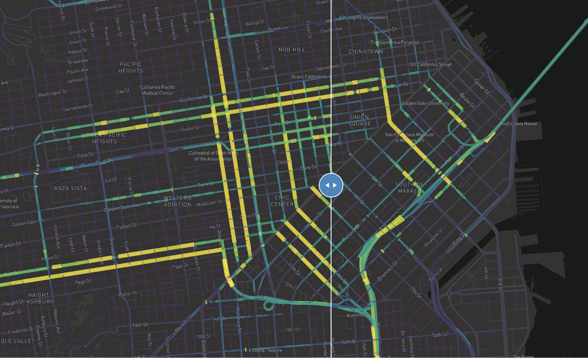
Above: Representative traffic volumes with data from before COVID19 on the left and after (on Monday, March 16) on the right. Interactive example site here.

Overview

The purpose of this document is to describe the data being produced and explain how to use it to create maps and graphics that can be used to share with the general public.

This dataset is based on the Mapbox telemetry data, and is intended to illustrate the changes in the driving patterns in a number of large cities over the course of the past few weeks. For each city and date, the dataset shows the normalized total number of vehicles on each road over the whole 24 hour period, for all roads where enough data was available to pass our privacy thresholds. This dataset does not contain any non-driving traffic, or any driving traffic not on publicly accessible roads.

For each site (city), we are producing the following information:

1. A “before” dataset for each day in the week consisting of the Sunday through Saturday period of January 12-18, 2020 with a traffic volume index value associated with each road segment in the target city.
2. For each day from Monday, March 16 onward (until end of project) an “after” dataset with a traffic volume index value associated with each road segment in the target city.

Using the two datasets, a map like the one in the screenshot shown above can be created. An example HTML document (the shared index.html file) is included to show how to parse the two above datasets and map them. This is also hosted as an example site here, too.

Read through the shared HTML file to see how the data is processed to make traffic volume index values between the before and the after datasets match each other. This, in conjunction with leveraging Mapbox style expressions, will allow one to generate maps such as the one above, in which the line width is a product of the traffic volume indices.

Note that it is not recommended to serve up the raw GeoJSON for larger sites or if multiple maps are being shown at once. Instead, we recommend a processing step on the consumer end (whoever is pulling from the bucket) whereby the data is compressed, converted to vector tiles, or filtered to smaller areas before ultimately being served up in a map for readers/the general audience. The reason for this is simply that larger and more dense (network-wise) cities ultimately produce signficantly larger amounts of data. As a result, file sizes can be large enough that they become burdensome on web pages, particularly if multiple sites or days are being loaded at once.

Explanation of data structure

The before and after datasets have the same structure - both are what is known as ndjson. That is, they are a data format where each line is an JSON object. Thus the composite file is a set of JSON objects separated by new line separators (thus “newline-delimited JSON”). In this case, each line is a GeoJSON which can be mapped directly onto a Mapbox map.

The above example shows the composition of a single line from one of these before or after datasets. The geometry key contains a coordinate array that can be used to map the shape onto the Mapbox map (which will handle the full feature if provided).

The vehicle_volume_index represents the normalized total number of vehicles on the road over the 24 hour period indicated in the file name. This value ranges from 0.00001 to infiniti, and can be used to compare the relative traffic volumes between dates or different roads: for example, a road with a vehicle_volume_index value of 0.2 will have seen exactly twice the number of cars per meter of road over a single 24 hour period as a road with a vehicle_volume_index of 0.1.

We normalize vehicle volume counts, instead of producing raw counts, in order to provide maximum user privacy protection. The process for generating the vehicle_volume_index is as follows:

1. We collect total raw car counts on each road over each 24 hour period
2. We apply a small randomized noise factor to each car count, and drop records for all roads where the total of (count cars + noise factor) was less than our minimum required privacy threshold.
3. We divide the number obtained in the previous step by a scaling factor. This scaling factor remains constant within each city over time, but may differ between cities. For example, a value of 2.028 at site one (say, San Francisco) is not equal to a value of 2.028 at site two (say, Miami). Thus, it is important to understand that vehicle_volume_index is a value that can only be used to compare vehicle_volume_index values between road segments within the context of a single site (in this case, a city).
4. We divide the resulting scaled counts by the length of the road in km. This ensures that long road segments don’t end up looking as extremely “high traffic” just because there is a higher probability that a car’s location will get sampled somewhere along the span of the road.

These indices have been created and are unique to each site. These indices have been created for privacy reasons and to protect the underlying total volume data that Mapbox contains.

We recommend, for the purposes of visualizing this data, further rescaling vehicle_volume_index to a scale between 0 and 1 for each site across the dates being compared. The resulting values can then be used as basis for the width and color of the lines on the map.

For example, in the shared index.html file, this value is created by first getting the maximum vehicle_volume_index value observed on a segment between both the before and the after data. This value is stored as a variable named denominator and is produced as the max value of the getDenominator() method when applied to the data from both the before and after data.

Once the denominator value is generated, each vehicle_volume_index is divided by it, thus creating the ratio value. Add this value to the property of each row and add all values into a parent GeoJSON FeatureCollection. This data can then be added to the source data for each of the before and after maps, thus allowing the road segments to be rendered.

We recommend using this method in all your applications of the data as well (it calculates the 98th percentile instead of the max, which avoids some edge cases that can occur with these indices).

Location of data

Data is stored on S3. While this project is occurring, a daily job will output data to a bucket on S3. This bucket has been shared with the AWS account of any participating 3rd parties. The permissions of the 3rd party are read-only.

The location of the bucket is: s3://telem-densities-sample-maps/. For each day, a target city’s traffic volume index data is published to this bucket. The structure of these files is described in the following section.

Format for accessing each date

Each day will be processed and posted to S3. This section describes the structure of the file name so that it can be programmatically extracted. Here is an example real file available on the bucket: 2020-03-16_oakland_traffic_volumes.geojson

The file name is composed of two parts: the date and the city name. To query for a file name, format a string in the following pattern: {YYYY-MM-DD}_{city_name_lowercase}_traffic_volumes.geojson

Note that while data for telemetry in the target sites is being produced daily during the quarantine period, a single week is produced for data before the quarantine. The reference week being used is the Sunday through Saturday period of January 12-18, 2020. This week period was identified as the last week before the coronavirus scare first hit and the last week before we saw drops in the amount of driving telemetry Mapbox collects.

Before data is stored in the same location but and with the same scheme. Since there is one dataset for each site for each day of the week from the reference January week, the dates for a Tuesday in March (for example, 2020-03-17) can be compared with a Tuesday before the quarantine period by using January date 2020-01-14. Thus, the before and after filenames for Houston would look like the following:

• Before: 2020-01-14_houston_traffic_volumes.geojson
• After: 2020-03-17_houston_traffic_volumes.geojson

Here is an example of a single week of data for all available sites:

Up and running with the example site

Simply download the sample site associated with this how-to guide (linked at top of page) that contains the static web page and 2 sample datasets. Place all 3 files in a directory and navigate into it via the command line. Start a simple HTTP server and navigate the localhost port address that you are serving to and you should be able to view and interact with the simple example site and data.